
The developers are happy to announce the release v0.5.0 of the optic design / simulation software OPOSSUM!
Over the past four releases, many concepts and features have been worked out. Meanwhile, the software can already be used for simulating real-life optical models. However, since the software still lacks a real user interface (it’s more like an optics library) and file / data formats are changing rapidly, using the software for real projects is still cumbersome and requires familiarity with the Rust programming language. If you are, nevertheless, willing to test the software, feel free to do so. We are open for feedback and we would be happy and thankful for any feature request or bug report. All bugs / feature requests should be reported to our software repository.
Here are the highlights of the v0.5.0 release:
1 Introduction of a geometry model
This release mainly focused on the development of a concise geometry model which involves the implementation of a global coordinate system and the positioning of optical elements in 3D space using isometric transformations. Furthermore, we worked out a concept for positioning nodes in a way that simply “works as expected” within the typical optical design workflow.
In contrast to other well-established design software solutions (e.g., ZEMAX or Code V) we wanted to avoid often confusing “coordinate breaks” as much as possible. For this, we make use of the old concept of an optical axis. While an optical axis can, strictly spoken, not always be concisely defined, it dramatically simplifies positioning and aligning optical elements. For the majority of optical systems, it is sufficient to simply define the distance between two optical elements and optionally a tilt or decenter. This allows for example to model the following optical setup which requires only two distances and two tilt angles:
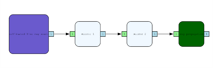
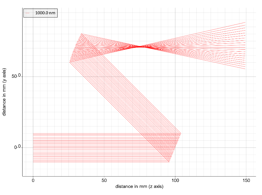
Figure 1: Optical system consisting of a source at the origin, a 22.5° tilted mirror at a distance of 100 mm from the source and a 22.5° tilted concave mirror with R=100 mm and a distance of 100 mm from the previous optic
The above model so can be modeled with less than 10 lines of (Rust) code.
Besides the above “relative” positioning, it is of course still possible to assign an absolute position / orientation to an optical element.
With the new geometry model and the usage of so-called “reference nodes” (a node referring to another existing node), it is also possible to model optical systems where beams can pass elements more than once.
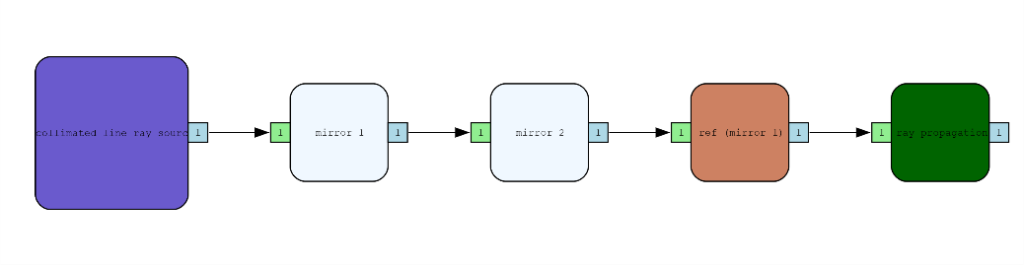
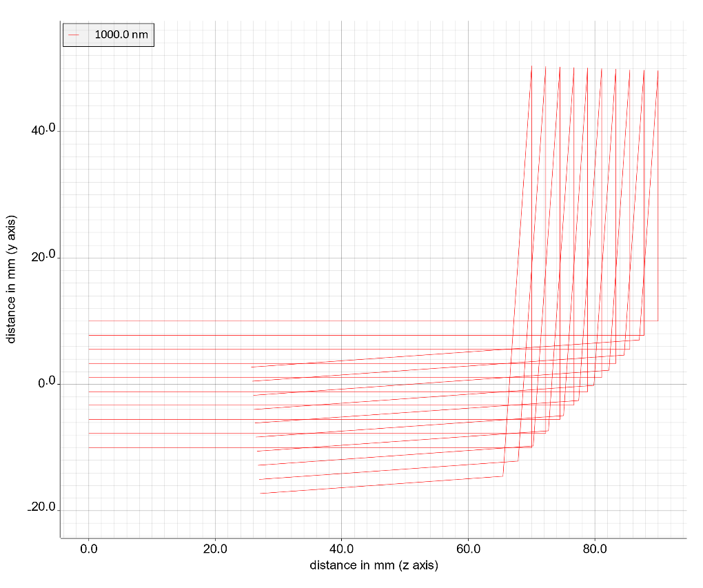
Figure 2: Optical system consisting of a source at the origin, a 45° tilted mirror and a 2° tilted mirror that redirects the rays onto the first mirror
In the above example, we use two mirrors with the second one tilted by only 2 °, thus hitting the first mirror again.
2 New optical elements
As shown above, the new release now includes flat and spherically curved mirrors. Furthermore, cylindric lenses have been added. Also wedged surfaces have been introduced which can be used as wedged windows or even prisms. This way it is now possible to model anamorphic prism pairs.
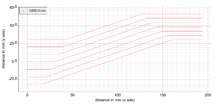
Figure 3: Example of an anamorphic prism pair
Note: So far, the optical elements are not yet displayed in the above beam propagation plots. This is on our to-do list…
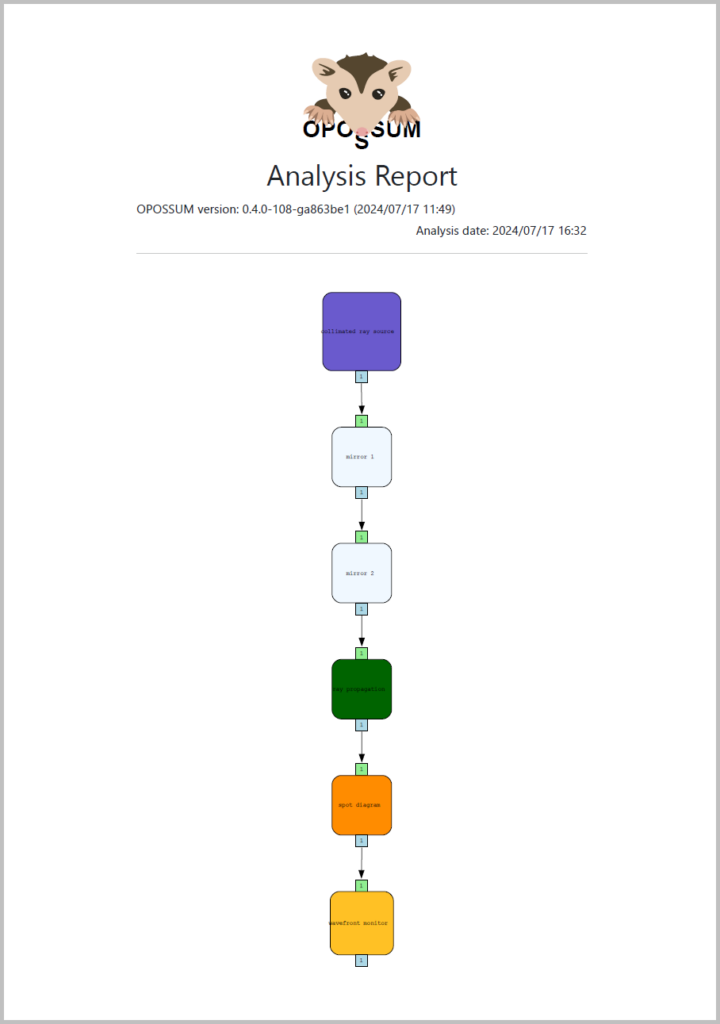
3 Improved analysis reports
While the past releases generated analysis reports in PDF format, we decided to switch to HTML reports for several reasons: The used PDF library had many dependencies on other software packages, which became increasingly tedious to manage. In addition, the formatting possibilities of this library were rather limited. The switch to an HTML report generation reduced the executable size by about 40 %.
The generated HTML report can be easily inspected using a simple web browser. To still generate a PDF document, almost all browsers offer the possibility to print the document to a PDF printer. There is still room for improvement of the layout / styling, which will be targeted in the next releases.
4 Support for ambient medium
With this release, a global ambient medium can be defined. By default, it is still defined as ‘vacuum’. However, it is now possible to define a new medium such as ‘air’ which is used for the propagation between the optical nodes.
5 Improved warnings during analysis
Warnings and error messages have been significantly improved in this release. For example, if you want to model an energy meter of a given detector size you define a corresponding input aperture (such as a circular or a rectangular area). During analysis, a warning is issued now if incoming rays miss this surface indicating that the measured energy might not be “the full story”.
6 Further improvements
Besides the above highlights, a lot of development work went into bug fixing and smaller improvements as well as a heavily extended test suite. Some statistics:
- 42 tickets closed
- > 300 repository commits
- > 580 unit tests
- > 90 % code coverage by unit tests
- > 30.000 lines of code
For the upcoming release, we will concentrate on the development of a new module for the automatic calculation of ghost foci in complex optical systems.
For more information, visit thrill-project.eu/opossum
Text: Udo Eisenbarth
